Introduction to R & RStudio

Abstract

This section provides a short introduction to and RStudio. It also touches differences between base R and the tidyverse package collection.

What is & RStudio?

• is a free software environment for statistical computing and graphics. It compiles and runs on a wide variety of UNIX platforms, Windows and MacOS (see https://www.r-project.org/).

• R Studio is a integrated development environment (IDE) for , built by Posit.

Some advertisement from the Posit website:

Used by millions of people weekly, the RStudio integrated development environment (IDE) is a set of tools built to help you be more productive with R and Python. It includes a console, syntax-highlighting editor that supports direct code execution. It also features tools for plotting, viewing history, debugging and managing your workspace.

Of course there are other IDEs (e.g., Visual Studio Code, or VIM), but if you use R, RStudio is most likely the way to go.

Positron a next-generation data science IDE

Posit recently released the beta version of a next-generation data science IDE named Positron, which could serve as a viable alternative to RStudio. It is also tailored for R but also supports seamless Python integration.

How to work with R and RStudio?

First step: Open RStudio!

This should look like this, maybe or probably with a different appearance (this is the Dracula theme).

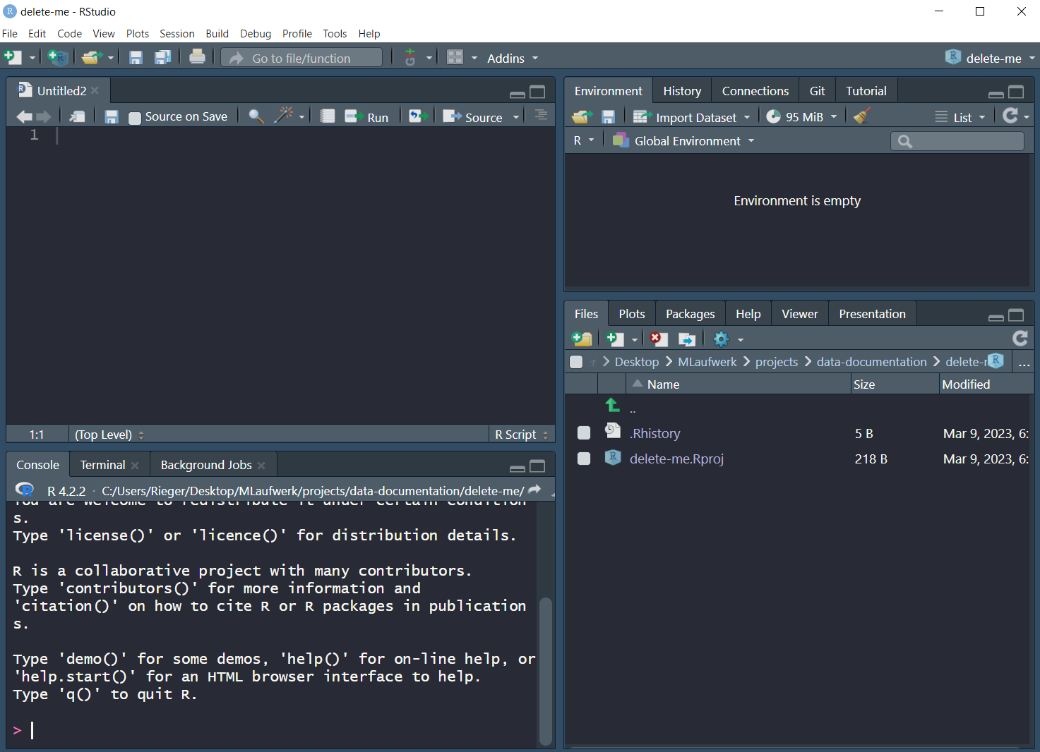
You can change the theme via Tools > Global Options > Appearance

In RStudio, there are four customizable panes. These can be configured by navigating to: Tools > Global Options > Pane Layout:

Panes

• Console
  • Here you can access R (but you should not, see the warning below)
  • E.g., ask R what is: 2 + 2
• Source/Script
  • Editor to save scripts

Warning

You should never work directly in the Console, but always use a R-script (e.g., script.R) or even better a Quarto document (e.g., script.qmd). It is important to understand and reproduce everything you did.

• Environment/History/…/Tutorial
  • Environment: contains all objects that were created or loaded during an R session
  • History:
  • … e.g., the free and open source distributed version control system git
  • Tutorial: A tutorial to learn R with the learnr package (Aden-Buie et al., 2023)
• Files/Plots/Packages/Help/Viewer
  • Files: is kind of the file manager
  • Plots: shows the generated plots
  • Packages: overview of the (loaded &) installed packages
  • Help: When you ask for help (e.g., regarding a specific function in R: ?mean)
  • Viewer: E.g., previewing rendered Quarto documents

Projects

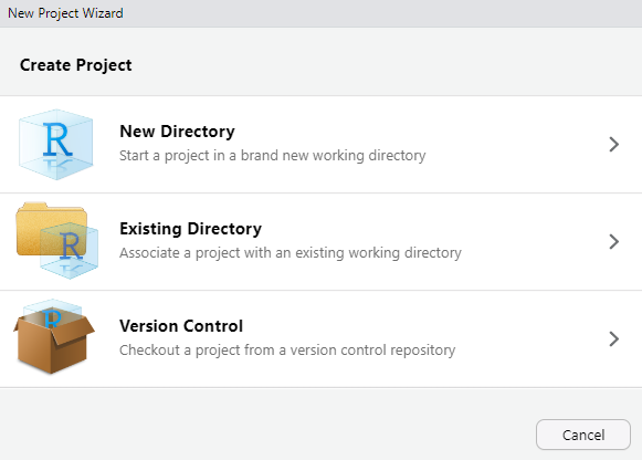
It is also advisable to use the project option. This means, whenever you start a new project (e.g., a data-related project), create an (R) project: File > New Project

Exercise: Create an project!

1. Choose between:

• New Directory (for now)

• Existing Directory

• Version Control (this is recommended, but is beyond the scope of this workshop)

2. Choose a project type (today a R project or Quarto project)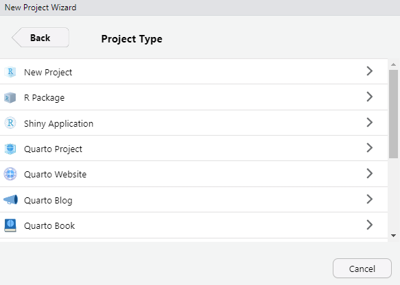

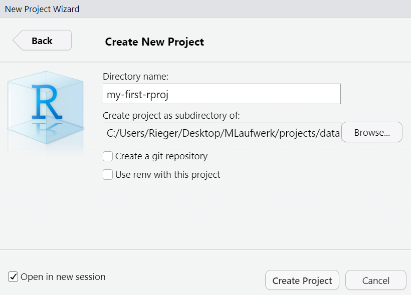
3. Provide a short name, set the check mark Open in new session and click Create Project

If you are interested in how to implement a reproducible project-oriented workflow, you might find this introduction helpful.

Short introduction to the R programming language

This section gives a (very?) brief introduction to the R programming language.

For (more) comprehensive introductions…

…or overviews of the language see (e.g.):

• R Manual on the CRAN website

• R for Data Science by Hadley Wickham and Garrett Grolemund

• Hands-On Programming with R by Garrett Grolemund

• Introduction to R by the IDRE Statistical Consulting Group

• …

To understand computations in R, two slogans are helpful:

• Everything that exists is an object.
  
• Everything that happens is a function call.

– John Chambers (creator of the S programming language)

Basics

Before working with R, there are a few basics you need to know:

• R is a case-sensitive programming language. This means that R distinguishes whether a word is written in upper or lower case

"name" == "Name"

[1] FALSE

• Values are assigned to objects using <-

a <- "Hello world!"

• Arguments within functions are assigned using =

df <- data.frame(
  x = 1:4,
  y = 3:6
)

Exercise: Create a new R script

File > New File > R Script or alternatively use the shortcut Ctrl+Shift+NCtrl+Shift+N

Then save the file File > Save or File > Save As (shortcut: Ctrl-SCtrl-S)

Data Types

The basic data types¹ in R are depicted in Table 1.

Table 1: Basic data types in

Type	Description	Value (example)
Numeric	Numbers with decimal value or fraction	3.7
Integer	Counting numbers and their additive inverses	2, -115
Character	aka string. Letters enclosed by quotes in the output.	"Hello World!","4"
Logical	boolean	TRUE, FALSE
Factor	Categorial data - Level: characteristic value as seen by R - Label: designation of the characteristic attributes	0, 1 male,female
Special	Missing values: unknown cell value Impossible values: not a number Empty values: known empty cell value	NA NaN NULL

Exercise: Use the class function to check the data type of an object!

x <- 10
class(x)

[1] "numeric"

y <- "Hello World"
class(y)

[1] "character"

Data Structures

R has a couple of different data structures² which are briefly described in the following subsections.

Vector

• one-dimensional array
  
• same data type
• e.g., c(45, 6, -83, 23, 61)

Tips for handling vectors

Create a vector with the c function

v <- c(45, 6, -83, 23, 61)
v

[1]  45   6 -83  23  61

Or a named vector…

vNam <- c(a = 45, b = 6, c = -83, d = 23, e = 61)
vNam

  a   b   c   d   e 
 45   6 -83  23  61 

Count the amount of items contained in vector

length(v)

[1] 5

Vector indexing (by position)

v[1]

[1] 45

v[-3]

[1] 45  6 23 61

Slicing vectors

v[3:5]

[1] -83  23  61

Generate regular sequences using seq function

seq(from = 0,
    to = 20,
    by = 2)

 [1]  0  2  4  6  8 10 12 14 16 18 20

Matrix

• two-dimensional
  
• same data type
• example see on the right

Tip 1: Tips for handling matrices

The matrix function creates a matrix from the given set of values

m <- matrix(data = c(1, 2, 3, 45, 36, 52),
            nrow = 2,
            ncol = 3,
            byrow = TRUE)
m

     [,1] [,2] [,3]
[1,]    1    2    3
[2,]   45   36   52

Slicing works also on matrices: m[row , column]

m[, 1:2]

     [,1] [,2]
[1,]    1    2
[2,]   45   36

List

• can contain elements of various data types
• often ordered collection of values
• one-indexed (indexing starts with 1)
• e.g., list("hi", 2, NULL)

Tips for handling lists

Create lists (with different elements, i.e., numbers and letters) with the list function

l1 <- list(1:5)
l2 <- list(letters[1:5])
l3 <- list(LETTERS[1:5])

Create a nested list…

l4 <- list(l1, l2, l3)

…or a named (nested) list

l4Nam <- list("Numbers" = l1,
              "SmallLetters" = l2,
              "CaptialLetters" = l3)

Access list or nested list elements

l4[2]

[[1]]
[[1]][[1]]
[1] "a" "b" "c" "d" "e"

l4[[2]][3]

[[1]]
NULL

Unlist the list to get vector which contains all the atomic components

unlist(l1)

[1] 1 2 3 4 5

unlist(l4)

 [1] "1" "2" "3" "4" "5" "a" "b" "c" "d" "e" "A" "B" "C" "D" "E"

Count amount of items contained in list

length(l4)

[1] 3

length(unlist(l4))

[1] 15

Data frame

• various columns
• different data types
• variables = columns
• observations = rows
• example see on the right

Tip 2: Tips for handling dataFrames

df <- data.frame(
  id = 1:4,
  age = c(12, 13, 12, 14),
  sex = c(1, 1, 2, 2)
)
df

  id age sex
1  1  12   1
2  2  13   1
3  3  12   2
4  4  14   2

Number of observations

nrow(df)

[1] 4

Show dimension (rows, columns) of dataframe

dim(df)

[1] 4 3

Column names

colnames(df)

[1] "id"  "age" "sex"

Show the first two rows of the dataframe

head(df, 2)

  id age sex
1  1  12   1
2  2  13   1

Structure of dataframe object

str(df)

'data.frame':   4 obs. of  3 variables:
 $ id : int  1 2 3 4
 $ age: num  12 13 12 14
 $ sex: num  1 1 2 2

Some descriptive statistics using the summary function (for more see Section Descriptive statistics and item analysis

summary(df)

       id            age             sex     
 Min.   :1.00   Min.   :12.00   Min.   :1.0  
 1st Qu.:1.75   1st Qu.:12.00   1st Qu.:1.0  
 Median :2.50   Median :12.50   Median :1.5  
 Mean   :2.50   Mean   :12.75   Mean   :1.5  
 3rd Qu.:3.25   3rd Qu.:13.25   3rd Qu.:2.0  
 Max.   :4.00   Max.   :14.00   Max.   :2.0  

Base vs. & tidyverse

Besides the functionality of base R (R Core Team, 2024), there is the so-called tidyverse (Wickham, 2023) within R. The tidyverse is a collection of R packages (see Figure 1) that “share an underlying design philosophy, grammar, and data structures” and are (specifically) designed for data science (see https://www.tidyverse.org/).

Figure 1: tidyverse package collection

Within the tidyverse package collection, the dplyr package (Wickham et al., 2023) provides a set of convenient functions for manipulating data. Together with the pipe operator %>% from the magrittr package (Bache & Wickham, 2022)), it is an extremely powerful approach to manipulate data in a clear and comprehensible way. The native³ R pipe |> was introduced with R v4.1.0.

What does the pipe operator |>?

The tidyverse style guide suggests using the pipe operator “to emphasize a sequence of actions”. The pipe operator can be understood as “take the object and then” pass it to the next function. In the following, the use of the base R pipe operator is shown:

1. Take the data frame exDat and then
2. Select the variables: msc1 and msc2 and then
3. Calculate descriptive statistics using the describe function from the psych package (Revelle, 2024) and then
4. Create a table with the kable function from the knitr package (Xie, 2023)

exDat |> 
  dplyr::select(c(msc1, msc2)) |>
  psych::describe(fast=TRUE) |> 
  knitr::kable(digits = 2) 

	vars	n	mean	sd	median	min	max	range	skew	kurtosis	se
msc1	1	750	2.52	0.74	3	1	4	3	-0.02	-0.31	0.03
msc2	2	680	2.54	0.72	3	1	4	3	-0.02	-0.27	0.03

In contrast, when we use a nested approach the code would look like this:

knitr::kable(psych::describe(exDat,fast=TRUE),digits = 2) 

…or maybe a little bit more clear:

knitr::kable(
  psych::describe(exDat,
                  fast=TRUE),
  digits = 2) 

Nevertheless, when there are many functions, it gets kind of messy and difficult to comprehend. For more information on how to use pipes, see Chapter 4 of the guide.

References

Aden-Buie, G., Schloerke, B., Allaire, J., & Rossell Hayes, A. (2023). Learnr: Interactive tutorials for r. https://rstudio.github.io/learnr/

Bache, S. M., & Wickham, H. (2022). Magrittr: A forward-pipe operator for r. https://magrittr.tidyverse.org

R Core Team. (2024). R: A language and environment for statistical computing. R Foundation for Statistical Computing. https://www.R-project.org/

Revelle, W. (2024). Psych: Procedures for psychological, psychometric, and personality research. https://personality-project.org/r/psych/ https://personality-project.org/r/psych-manual.pdf

Wickham, H. (2023). Tidyverse: Easily install and load the tidyverse. https://tidyverse.tidyverse.org

Wickham, H., François, R., Henry, L., Müller, K., & Vaughan, D. (2023). Dplyr: A grammar of data manipulation. https://dplyr.tidyverse.org

Xie, Y. (2023). Knitr: A general-purpose package for dynamic report generation in r. https://yihui.org/knitr/

Footnotes

1. We omitted the complex type.

2. We omitted arrays.

3. for the difference between |> and %>% see https://ivelasq.rbind.io/blog/understanding-the-r-pipe/