6  Import, merge & reshape data

This part provides an introduction to import, merge and reshape data sets with R.

6.1 Import (or export) data sets

In R data sets are usually stored as data.frame objects (see also the section Data Structures). There are other object types for data sets such as tibble from the tibble package (Müller & Wickham, 2023) or data.table from the data.table package (Dowle & Srinivasan, 2023) which are more efficient, especially when it comes to (very) large data sets (see e.g., Chapter 10 of R for Data Science and the vignette of the data.table package).

6.1.1 Data frames

Data sets can come in many different file formats. For example, .txt, .csv files, or .sav (SPSS), dta (Stata), .sas7bdat (SAS) files.

To import e.g., .csv or .txt files, R offers a couple of functions that deal with these formats:

• utils::read.table: Reads a file in table format and creates a data frame from it, with cases corresponding to lines and variables to fields in the file.

  • utils::read.csv or utils::read.csv2¹
  • utils::read.delim or utils::read.delim2

• base::readLines: Read some or all text lines from a connection.

• …

When it comes to other (software specific) formats, you need additional packages e.g., foreign (R Core Team, 2022) or haven (Wickham et al., 2022).

To import the SPSS data sets (.sav file), we may use the read.spss function from the foreign package (R Core Team, 2022). There are a couple of default arguments which you (likely) want to change:

• use.value.labels: logical: convert variables with value labels into R factors with those levels? (default is TRUE switch to FALSE)
• to.data.framelogical: return a data frame? (default is FALSE switch to TRUE)
• use.missings: logical: should information on user-defined missing values be used to set the corresponding values to NA?

exDatImpforeign <- foreign::read.spss("path-to-file.sav-file",
                                      use.value.labels = FALSE,
                                      to.data.frame = TRUE,
                                      use.missings = TRUE)

Exporting dataframes

To export data to a file, you can use the base::write function(s):

• utils::write.table
• utils::write.csv or utils::write.csv2
• …

Again, when it comes to software-specific file formats you need additional packages such as foreign (R Core Team, 2022) or haven (Wickham et al., 2022):

• haven::write_sav
• foreign::write.foreign
• …

In the following, the use of the write.foreign function is displayed:

getwd()
codefile <- tempfile()

foreign::write.foreign(exDat,
                       "exDat.sav",
                       codefile = codefile,
                       package = c("SPSS"))

unlink(codefile)

Note that there are a couple of further steps necessary to get a working .sav file. We recommend using the haven (Wickham et al., 2022) package (see below), at least when it comes to exporting data sets.

6.1.2 Tibbles

The tibble package is part of the tidyverse² (Wickham, 2023).

First, check the class of the example data set exDat.

class(exDat)

[1] "data.frame"

The as_tibble function from the tibble package (Müller & Wickham, 2023) turns an existing object (a data frame or matrix) into tibble which is a data.frame variant (with nice defaults) and class tbl_df (see ?tibble::as_tibble).

exDatTib <- tibble::as_tibble(exDat)
class(exDatTib)

[1] "tbl_df"     "tbl"        "data.frame"

The write_sav function from the haven package (Wickham et al., 2022) can also be used to export data sets. Before exporting the data, you may want to check your working directory with the getwd() function.

getwd()
haven::write_sav(exDat, "exDat.sav")

To import the data set, we use the read_sav function from the haven package.

exDatImpTest <- haven::read_sav("exDat.sav")

Note that the read_sav returns a tibble, data.frame variant (with nice defaults).

For more see https://tibble.tidyverse.org/ and Chapter 10 of R for Data Science.

6.2 Merge data sets

Merging data sets is necessary, because we often work with different data sources. By merging, we combine the information from multiple data sets to create one (complete) data set.

Before we merge, we need another data set. Execute the following code to simulate one!

PopModGSC <- "
eta2 =~ .8*gsc1 + .8*gsc2 + .8*gsc3 + .8*gsc4
eta2 ~~ 1*eta2
eta2 ~ 0*1

gsc1 | -1.5*t1 + 0*t2 + 1.5*t3
gsc2 | -1.5*t1 + 0*t2 + 1.5*t3
gsc3 | 1.5*t1 + 0*t2 + -1.5*t3
gsc4 | 1.5*t1 + 0*t2 + -1.5*t3

"

exDatGSC <- lavaan::simulateData(model = PopModGSC,
                                 sample.nobs = 700,
                                 seed = 999)
exDatGSC$id <- 1:nrow(exDatGSC)

base R

The merge function is designed to merge two data frames by common columns or row names, or do other versions of database join operations. It requires at least two input arguments x,y that are data frames, or objects to be coerced to one. However, it is recommended to provide some more information by using the further input arguments, including:

• by, by.x, by.y: specifications of the columns used for merging. See ‘Details’.

• all: logical; all = L is shorthand for all.x = L and all.y = L, where L is either TRUE or FALSE.

• all.x: logical; if TRUE, then extra rows will be added to the output, one for each row in x that has no matching row in y. These rows will have NAs in those columns that are usually filled with values from y. The default is FALSE, so that only rows with data from both x and y are included in the output.

• all.y: logical; analogous to all.x.

• …

exDatComb <- merge(exDat, exDatGSC,
                   by = "id",
                   all.x = TRUE)
head(exDatComb)

  id msc1 msc2 msc3 msc4       age sex edu  fLang gsc1 gsc2 gsc3 gsc4
1  1    2    3    2    2  9.815538   0   0 german    3    3    2    3
2  2    3    2    1    1  8.980194   1   0 german    3    3    3    4
3  3    2    2    3    3 12.758157   0   0 german    2    1    2    2
4  4    2    2    3    2 10.578846   0   0 german    2    2    3    3
5  5    3    2    2    2  9.894364   1   0 german    3    3    2    3
6  6    3    3    3    2 10.446850   0   0 german    2    3    3    3

dplyr package

In the dplyr packages, there are 4 functions that are designed to combine data sets which need two input arguments x and y:

1. dplyr::left_join keeps all observations in x.

2. dplyr::right_join keeps all observations in y.

3. dplyr::inner_join only keeps observations from x that have a matching key in y.

4. dplyr::full_join keeps all observations in x and y.

It is recommended to use the by argument to specify the column(s) that are used for joining/merging.

exDat |>
  dplyr::left_join(exDatGSC, by = "id") |>
  head()

  msc1 msc2 msc3 msc4       age sex edu  fLang id gsc1 gsc2 gsc3 gsc4
1    2    3    2    2  9.815538   0   0 german  1    3    3    2    3
2    3    2    1    1  8.980194   1   0 german  2    3    3    3    4
3    2    2    3    3 12.758157   0   0 german  3    2    1    2    2
4    2    2    3    2 10.578846   0   0 german  4    2    2    3    3
5    3    2    2    2  9.894364   1   0 german  5    3    3    2    3
6    3    3    3    2 10.446850   0   0 german  6    2    3    3    3

If you need to quickly save an object (e.g., a data set like exDatComb), you may use the base::saveRDS function.

#getwd()
saveRDS(exDatComb,
        "exDatComb.RDS")

6.3 Reshape data

Reshaping data refers to the process of transforming the structure of data. Two popular ways of structuring data sets are the so-called wide and long data format. In Table 6.1 an example longitudinal data set is depicted in the wide and long format.

Table 6.1: Example (longitudinal) data set in the…

(a) …wide format

PID	\(Y_1\)	\(Y_2\)	\(\dots\)	\(Y_t\)
1	3	4
2	2	2
3	1	4
4	4	1
\(\vdots\)
N

(b) …long format

PID	\(Y\)	Time
1	3	0
1	4	1
2	2	0
2	2	1
\(\vdots\)
4	4	0
4	1	1
\(\vdots\)		\(\vdots\)
N		t

• Wide data format
  • rows = repeated measurements of 1 unit in separate columns
    
  • columns = (time-point-)specific variables (i.e., \(Y_{1}\), \(Y_{2}\), \(\dots\), \(Y_{t}\))
• Long data format
  • rows = one (time-point-)specific measurement per unit
  • columns = multiple variables collapsed into a single column (i.e., \(Y\))

Another data scenario in which you may want to reshape your data is when the goal is to examine or visualize (see below) multiple items of a scale. This is the working example.

base R

The reshape function from base R is designed to transform data sets between wide and long format. The following arguments are recommended to use:

• data: a data frame
• varying: names of sets of variables in the wide format that correspond to single variables in long format (‘time-varying’). This is canonically a list of vectors of variable names, but it can optionally be a matrix of names, or a single vector of names. In each case, when direction = "long", the names can be replaced by indices which are interpreted as referring to names(data). See ‘Details’ for more details and options.
• v.names: names of variables in the long format that correspond to multiple variables in the wide format. See ‘Details’.
• timevar: the variable in long format that differentiates multiple records from the same group or individual. If more than one record matches, the first will be taken (with a warning).
• times: the values to use for a newly created timevar variable in long format. See ‘Details’.
• direction: character string, partially matched to either "wide" to reshape to wide format, or "long" to reshape to long format.

Now we transform the example data set exDat to the long format…

exDatLong <- reshape(exDat,
                     varying = names(mscItems),
                     v.names = "value",
                     timevar = "Item",
                     times = names(mscItems),
                     idvar = "id",
                     direction = "long")

head(exDatLong[sort(exDatLong$id),], 10)

               age sex edu  fLang id Item value
1.msc1    9.815538   0   0 german  1 msc1     2
1.msc1.1  9.815538   0   0 german  1 msc1     2
1.msc1.2  9.815538   0   0 german  1 msc1     2
1.msc1.3  9.815538   0   0 german  1 msc1     2
2.msc1    8.980194   1   0 german  2 msc1     3
2.msc1.1  8.980194   1   0 german  2 msc1     3
2.msc1.2  8.980194   1   0 german  2 msc1     3
2.msc1.3  8.980194   1   0 german  2 msc1     3
3.msc1   12.758157   0   0 german  3 msc1     2
3.msc1.1 12.758157   0   0 german  3 msc1     2

… and back to to the wide format.

exDatWide <- reshape(exDatLong,
                     varying = names(mscItems),
                     v.names = "value",
                     timevar = "Item",
                     idvar = "id",
                     direction = "wide")
head(exDatWide, 10)

              age sex edu  fLang id msc1 msc2 msc3 msc4
1.msc1   9.815538   0   0 german  1    2    3    2    2
2.msc1   8.980194   1   0 german  2    3    2    1    1
3.msc1  12.758157   0   0 german  3    2    2    3    3
4.msc1  10.578846   0   0 german  4    2    2    3    2
5.msc1   9.894364   1   0 german  5    3    2    2    2
6.msc1  10.446850   0   0 german  6    3    3    3    2
7.msc1  10.897605   1   0 german  7    4    4    1    2
8.msc1   7.977382   1   0 german  8    3    3    2    1
9.msc1  10.688379  NA   0 german  9    3    3    2    1
10.msc1  9.105864   0   0 german 10    3    3    2    2

#exDatWide[,paste0("msc",1:4)] == exDat[,paste0("msc",1:4)]

tidyr package

Within the tidyverse the tidyr package (Wickham et al., 2023) offers two functions that are designed to transform the data to wide (pivot_longer) or long (pivot_wider) format.

tidyr::pivot_longer “lengthens” data, increasing the number of rows and decreasing the number of columns. The function requires only the cols statement, although the names_to and values_to arguments are recommended).

exDatLong2 <- exDat |>
  tidyr::pivot_longer(cols = names(mscItems),
                      names_to = "Item",
                      values_to = "value")

head(exDatLong2, 10)

# A tibble: 10 × 7
     age   sex   edu fLang     id Item  value
   <dbl> <dbl> <dbl> <chr>  <int> <chr> <dbl>
 1  9.82     0     0 german     1 msc1      2
 2  9.82     0     0 german     1 msc2      3
 3  9.82     0     0 german     1 msc3      2
 4  9.82     0     0 german     1 msc4      2
 5  8.98     1     0 german     2 msc1      3
 6  8.98     1     0 german     2 msc2      2
 7  8.98     1     0 german     2 msc3      1
 8  8.98     1     0 german     2 msc4      1
 9 12.8      0     0 german     3 msc1      2
10 12.8      0     0 german     3 msc2      2

tidyr::pivot_wider “widens” data, increasing the number of columns and decreasing the number of rows. The function requires the value_from and names_from arguments (id_cols statement is recommended).

exDatWide2 <- exDatLong2 |>
  tidyr::pivot_wider(values_from = "value",
                     names_from = "Item",
                     id_cols = "id")
head(exDatWide2, 10)

# A tibble: 10 × 5
      id  msc1  msc2  msc3  msc4
   <int> <dbl> <dbl> <dbl> <dbl>
 1     1     2     3     2     2
 2     2     3     2     1     1
 3     3     2     2     3     3
 4     4     2     2     3     2
 5     5     3     2     2     2
 6     6     3     3     3     2
 7     7     4     4     1     2
 8     8     3     3     2     1
 9     9     3     3     2     1
10    10     3     3     2     2

Why reshaping to the long format? A visualization of likert scale data.

0. Load ggplot2

library(ggplot2)

1. Calculate frequencies with the base::table function (per Item) and store them in a new data set (here: mscPlot).

mscPlot <- as.data.frame( with(exDatLong, table(Item, value)) )

2. Visualize the frequencies using ggplot2.

ggplot(data = mscPlot,
       aes(x = factor(Item,
                      labels = stringr::str_wrap(mscItems, 35)), # break lines after 35 chr
           y = Freq,
           fill = value)) +
  geom_col(position="fill") + # bar chart
  scale_fill_brewer(palette = "Set2" # cosmetics start here
                    ,labels = c("1 = trifft überhaupt nicht zu",
                                "2 = trifft eher nicht zu",
                                "3 = trifft eher zu",
                                "4 = trifft völlig zu")
                    ) +
  scale_y_continuous("Frequencies",
                     labels = scales::percent_format(scale = 100)) + # scales package for %
  scale_x_discrete("") +
  coord_flip() +
  theme_classic() +
  theme(legend.position = "top",
        legend.title = element_blank()) +
  guides(fill=guide_legend(nrow=2,byrow=TRUE))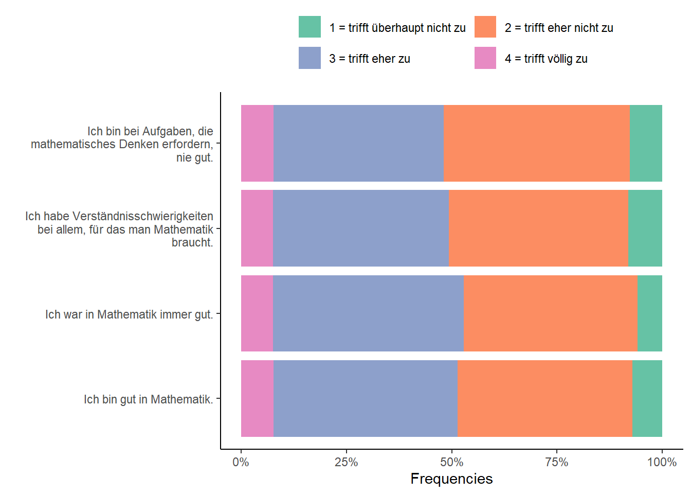

Dowle, M., & Srinivasan, A. (2023). Data.table: Extension of ‘data.frame‘. https://CRAN.R-project.org/package=data.table

Müller, K., & Wickham, H. (2023). Tibble: Simple data frames. https://CRAN.R-project.org/package=tibble

R Core Team. (2022). Foreign: Read data stored by minitab, s, SAS, SPSS, stata, systat, weka, dBase, ... https://svn.r-project.org/R-packages/trunk/foreign/

Wickham, H. (2023). Tidyverse: Easily install and load the tidyverse. https://CRAN.R-project.org/package=tidyverse

Wickham, H., Miller, E., & Smith, D. (2022). Haven: Import and export SPSS, stata and SAS files. https://CRAN.R-project.org/package=haven

Wickham, H., Vaughan, D., & Girlich, M. (2023). Tidyr: Tidy messy data. https://CRAN.R-project.org/package=tidyr

---

1. see also here: https://stackoverflow.com/questions/22970091/difference-between-read-csv-and-read-csv2-in-r

2. for more see the section on Base R vs. & tidyverse.