| X | Y | \(\overline{X}\) | \(\overline{Y}\) |
|---|---|---|---|
| 1 | 1 | 3 | 2.2 |
| 2 | 3 | 3 | 2.2 |
| 3 | 1 | 3 | 2.2 |
| 4 | 5 | 3 | 2.2 |
| 5 | 1 | 3 | 2.2 |
11 Correlation Analysis
Abstract
This chapter introduces correlation analysis and how to compute it using R.
NoteThis is work in progress…
Comming soon…
11.1 What is a Correlation?
In statistics, correlation is a type of statistical relationship between two random variables or bivariate data. It usually refers to the extent to which a pair of quantities are linearly related. More generally, an arbitrary relationship between variables is called an association, meaning the degree to which the variability in one can be accounted for by the other. […]
Definition retrieved from Wikipedia on May, 21, 2026.
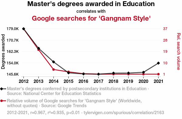
11.2 Correlation \(\neq\) Causation
11.3 Overview of Correlation Coefficients
Different types of correlation coefficients exist depending on the scale level and distributional properties of the variables:
- Pearson’s product moment correlation
- Spearman’s rank correlation coefficient
- Kendall’s \(\tau\)
- Cramér’s V
- Tetrachoric correlation
- Polychoric correlation
- …
11.4 Pearson’s product moment correlation coefficient
The Pearson’s product moment correlation coefficient is a statistical measure of the linear relationship between two (continuous) random variables. The formula is given in Equation 11.1.
\[ COR(X,Y) = \frac{COV(X,Y)}{SD_XSD_Y} = \frac{\frac{1}{n-1} \sum\limits_{i=1}^{n} (x_i - \bar{x})(y_i - \bar{y})}{\sqrt{\frac{1}{n-1} \sum\limits_{i=1}^n (x_i - \bar{x})^2}\sqrt{\frac{1}{n-1} \sum\limits_{i=1}^n (y_i - \bar{y})^2}} \tag{11.1}\]
The values range from -1 (perfect negative linear) to +1 (perfect positive linear).
The null hypothesis (usually) is \(H_0: \rho = 0\)
The formula of the test statistic is given in Equation 11.2.
\[ t = \frac{COR \cdot \sqrt{n-2}}{\sqrt{1-COR^2}} \qquad \text{ with } df = n-2 \tag{11.2}\]
11.5 Hand-calculation
CautionExercise
Calculate the Pearson’s product moment correlation coefficient for the following data by hand.
Use the formula(s) provided in Equation 11.1 (i.e., \(COV\), \(SD_X\), \(SD_Y\)).
11.5.1 Step 1: Calculate the Covariance
\[ \begin{aligned} COV_{XY} &= \frac{1}{n-1} \sum_{i=1}^{n} (x_i-\bar{x})(y_i-\bar{y}) \\[0.5em] &= \frac{ (1-3) \cdot (1-2.2) + (2-3) \cdot (3-2.2) + (3-3) \cdot (1-2.2) }{ 4 } \\ &\quad + \frac{ (4-3) \cdot (5-2.2) + (5-3) \cdot (1-2.2) }{ 4 } \\[0.5em] &= 0.5 \end{aligned} \]
11.6 Step 2: Calculate the Standard Deviations
\[ \begin{aligned} SD_X &= \sqrt{\frac{1}{n-1} \sum\limits_{i=1}^n (x_i - \bar{x})^2} \\&= \sqrt{\frac{(1-3)^2+(2-3)^2+(3-3)^2+(4-3)^2+(5-3)^2}{4}} \\&= 1.58 \end{aligned} \]
\[ \begin{aligned} SD_Y &= \sqrt{\frac{1}{n-1} \sum\limits_{i=1}^n (y_i - \bar{y})^2} \\&= \sqrt{\frac{(1-2.2)^2+(3-2.2)^2+(1-2.2)^2+(5-2.2)^2+(1-2.2)^2}{4}} \\&= 1.79 \end{aligned} \]
11.7 Step 3: Calculate the Pearson’s Correlation Coefficient
\[ \begin{aligned} COR_{XY} &= \frac{COV(X,Y)}{SD_XSD_Y} \\ &= \frac{0.5}{1.58 \cdot 1.79} \\& = 0.18 \end{aligned} \]